강사님 피드백 참고, 팀에서 알아본 데이터셋 취합 후 원하는 데이터들을 이용해 각자 eda 해보기로 함
0. 기본 세팅
import pandas as pd
import numpy as np
import copy
import datetime as dt

import seaborn as sns
import matplotlib.pyplot as plt

from sklearn.model_selection import train_test_split
from sklearn.cluster import KMeans
from sklearn.preprocessing import StandardScaler, MinMaxScaler
from sklearn.linear_model import LinearRegression

import matplotlib.font_manager as fm

font_path = 'C:\\Windows\\Fonts\\NanumBarunGothicLight.ttf'
font = fm.FontProperties(fname=font_path).get_name()
plt.rc('font', family='NanumBarunGothic')

pd.set_option('display.max_columns', None)
# pd.reset_option('display.max_columns')

1. 연령별 데이터
1-1. 데이터 로드
# folder = 'C:\\Users\\Y\\Desktop\\데이터분석_미니프로젝트\\data\\인구\\'
age_df = pd.read_excel(folder + '월별_매입자연령대별_아파트매매거래_동호수_수정_시트나눔.xlsx', sheet_name=None, engine='openpyxl')
age_df = pd.concat([value.assign(sheet_source=key) for key,value in age_df.items()], ignore_index=True)
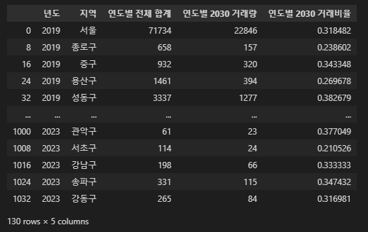
age_2030 = age_df[['sheet_source', '지 역', '매입자연령대', '연도별 전체 합계', '연도별 2030 거래량','연도별 2030 거래비율']]
age_2030 = age_2030[age_2030['연도별 2030 거래량'].notnull()]
age_2030['연도별 2030 거래량'] = age_2030['연도별 2030 거래량'].astype(int)
age_2030.rename(columns={'sheet_source':'년도', '지 역':'지역'}, inplace=True)
del age_2030['매입자연령대']
1-2. 그래프 양상
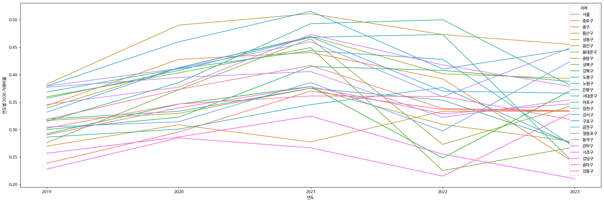
여기선,,,아무것도 못 봐,,,,,,
1-3. 서울, 노원구 제외
# age_2030['지역'].unique()
>> array(['서울', '종로구', '중구', '용산구', '성동구', '광진구', '동대문구', '중랑구', '성북구',
       '강북구', '도봉구', '노원구', '은평구', '서대문구', '마포구', '양천구', '강서구', '구로구',
       '금천구', '영등포구', '동작구', '관악구', '서초구', '강남구', '송파구', '강동구'],
      dtype=object)


# 서울, 노원구 제외
area = ['종로구', '중구', '용산구', '성동구', '광진구', '동대문구', '중랑구', '성북구',
       '강북구', '도봉구', '은평구', '서대문구', '마포구', '양천구', '강서구', '구로구',
       '금천구', '영등포구', '동작구', '관악구', '서초구', '강남구', '송파구', '강동구']
노원구와 각 자치구 연도별 2030 거래비율 양상 비교
# 노원구와 각 자치구 연도별 2030 거래비율 양상 비교
fig, axes = plt.subplots(nrows=12, ncols=2, figsize=(30, 25))

for row in range(12):
    for col in range(2):
        idx = row * 2 + col

        if idx < len(area):
            ax = axes[row][col]
            area_idx = area[idx]
            sns.lineplot(age_2030[age_2030['지역'].isin(['노원구', area_idx])], x='년도', y='연도별 2030 거래비율', hue='지역', ax=ax)
            ax.set(xlabel=area_idx)
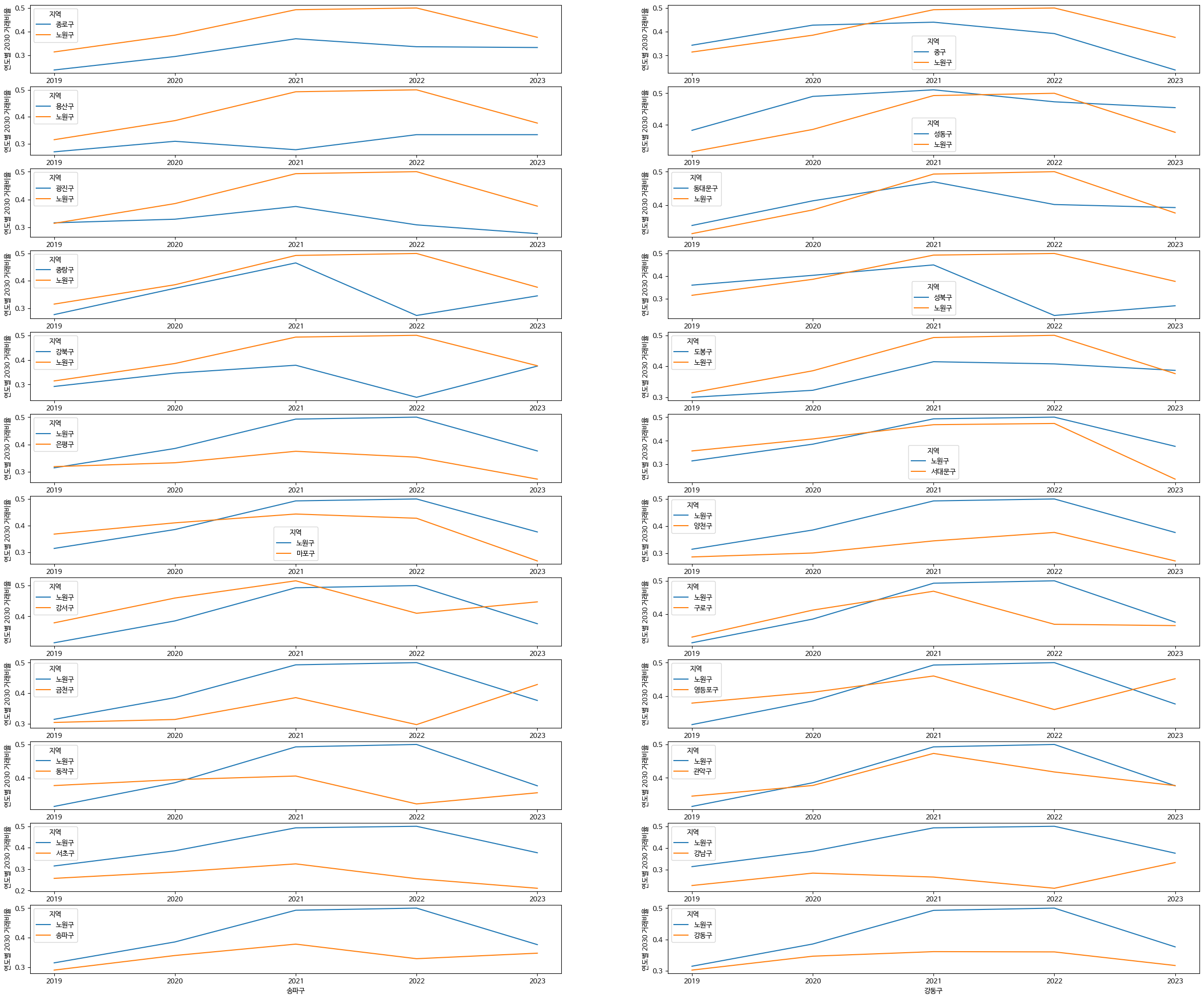
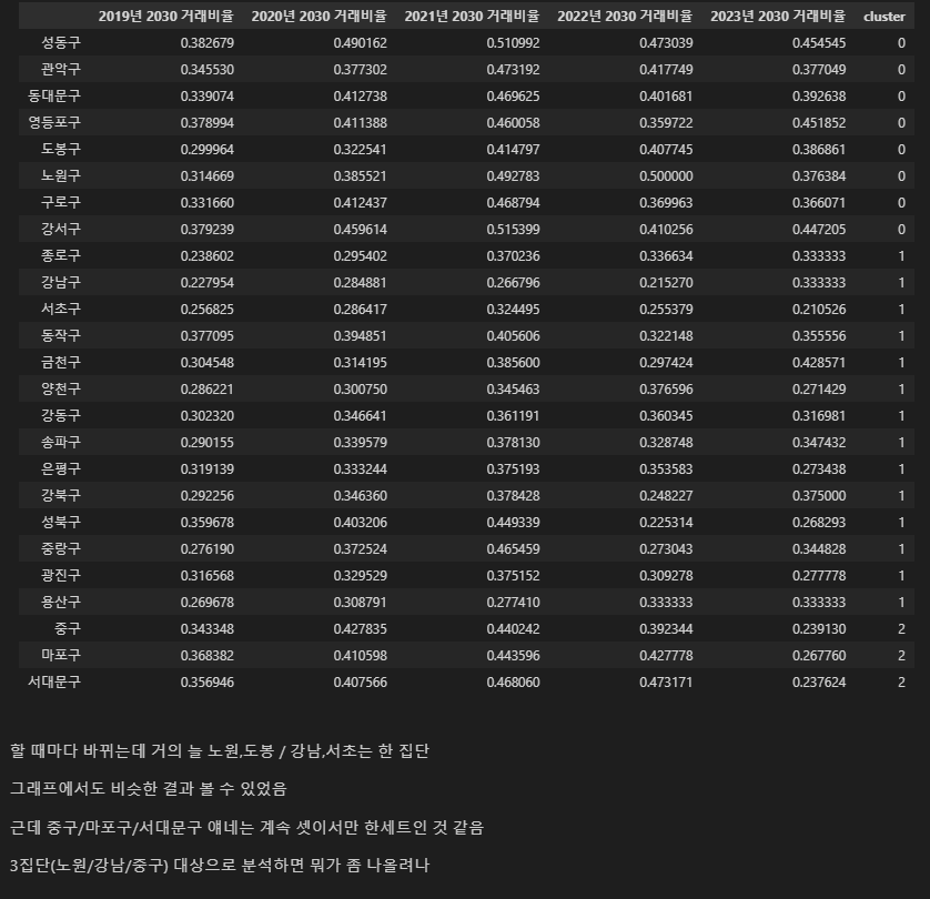
일단 얘 마음 속에 넣어놓구 클러스터링 진행
1-4. 클러스터링
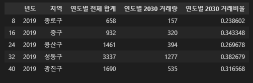
# 서울 제외
age_2030_tmp = age_2030[age_2030['지역'] != '서울']
age_2030_tmp.head()
# 시계열클러스터링 가능한 패키지 있긴 한데 과해서 그냥 df 만듦
rate_df = pd.DataFrame(index=[age_2030_tmp['지역'].unique()])

for i in range(2019, 2024):
    for area in age_2030_tmp['지역'].unique():
        rate_df.loc[area, f'{i}년 2030 거래비율'] = age_2030_tmp[(age_2030_tmp['년도']==str(i)) & (age_2030_tmp['지역']==area)]['연도별 2030 거래비율'].values

rate_df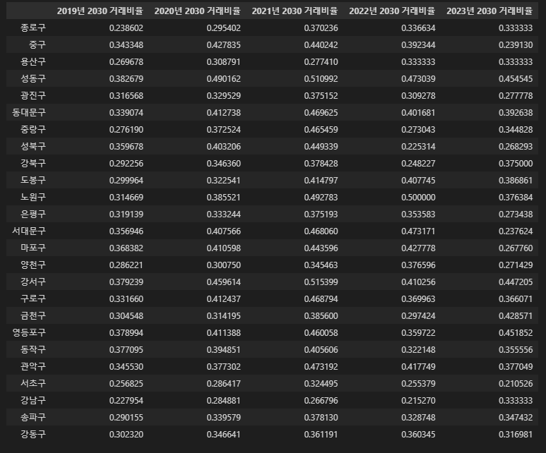
KMeans 이용
# kmeans 이용해 클러스터링
# 일단은 3개로
# from sklearn.cluster import KMeans
kmeans = KMeans(n_clusters=3)
clusters = kmeans.fit(rate_df)

# 그룹 번호 추출해서 cluster열에 저장
rate_df['cluster'] = clusters.labels_
rate_df.sort_values('cluster')
2. 관심 자치구 실거래가 데이터 이용
http://rtdown.molit.go.kr/
rtdown.molit.go.kr
2.1 데이터 로드
1년씩만 조회되길래 for문으로 데이터 불러와서 합치기,,,

# 데이터 로드
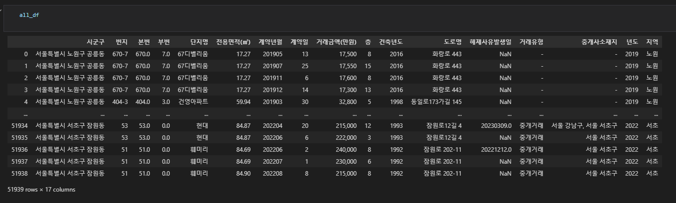
area = ['노원', '도봉', '강남', '서초']
all_df = pd.DataFrame()
for i in range(2019, 2023):
for j in area:
tmp = pd.read_excel(folder + f'아파트(매매)_실거래가_{j}_{i}.xlsx')
tmp['년도'] = i
tmp['지역'] = j
all_df = pd.concat([all_df, tmp]).reset_index(drop=True)
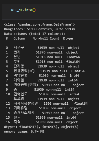
2-2. 스케일링
각 컬럼(면적, 거래 금액, 건축년도, 층)의 값들이 천차만별이라 스케일링 해버림
자치구끼리 비교하려는데 건축년도, 층 등의 컬럼은 필요없다고 생각했지만,,, 매입자 연령대가 다른 요인에 비해 미치는 영향이 큰지 알고 싶었기 때문에 일단 진행했음
MinMaxScaler 이용
# 스케일링
# from sklearn.preprocessing import StandardScaler, MinMaxScaler

scale_target = all_df[['전용면적(㎡)','거래금액(만원)','층', '건축년도']]
scale_target['거래금액(만원)'] = scale_target['거래금액(만원)'].replace(',','',regex=True).astype(int)
scaler = MinMaxScaler()

scaled = scaler.fit_transform(scale_target)
scaled_df = pd.DataFrame(scaled, columns=scale_target.columns)


scaled_df = pd.concat([all_df[['지역', '년도']], scaled_df], axis=1)
scaled_df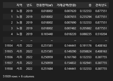
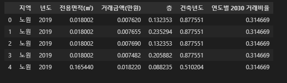
3. 연도별 2030 거래비율 join
# 연도별 2030 거래비율 join
age_2030['지역'] = age_2030['지역'].str[:2]
age_2030['년도'] = age_2030['년도'].astype(int)
basic_df = pd.merge(scaled_df, age_2030[['년도', '지역', '연도별 2030 거래비율']], on=['년도', '지역'], how='left')
basic_df.head()
4. 상관관계(상관계수)
corr 이용, heatmap 그림
corr = basic_df.corr()
sns.heatmap(corr, cmap='YlGnBu', annot=True)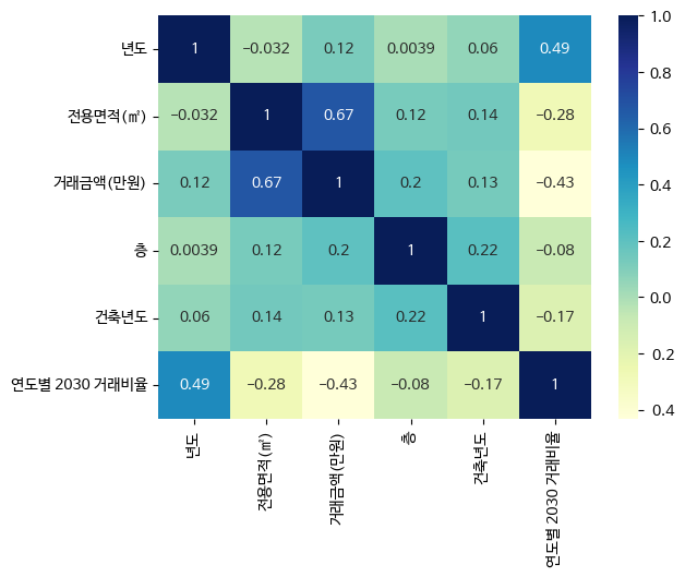
그래도 꽤 계수 절대값이 큼
5. 다중 선형 회귀 - 가중치 확인
# 회귀
# 데이터가 좀 있어서 train, test set 나눠도 될 것 같음
# from sklearn.model_selection import train_test_split
# from sklearn.linear_model import LinearRegression
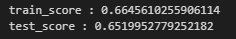
5-1. 일단 노원부터
# 노원
area = '노원'
data = basic_df[basic_df['지역']==area]

x = data[['년도', '전용면적(㎡)', '층', '건축년도', '연도별 2030 거래비율']]
y = data['거래금액(만원)']
x_train, x_test, y_train, y_test = train_test_split(x, y, train_size=0.8, test_size=0.2)

model = LinearRegression()
model.fit(x_train, y_train)

print('train_score :', model.score(x_train, y_train))
print('test_score :', model.score(x_test, y_test))
가중치 확인
# 가중치의 값은 coef_에 담겨있음
model.coef_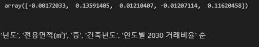
상수값
# 상수값
model.intercept_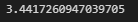
5-2. 노원 도봉, 서초, 강남
# 계수 담을 df
coef = pd.DataFrame(index=['노원', '도봉', '서초', '강남'], columns=x.columns)
coef.loc[area, :] = model.coef_
coef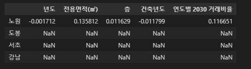
나머지도 선형 회귀 진행
# 도봉
area = '도봉'
data = basic_df[basic_df['지역']==area]

x = data[['년도', '전용면적(㎡)', '층', '건축년도', '연도별 2030 거래비율']]
y = data['거래금액(만원)']
x_train, x_test, y_train, y_test = train_test_split(x, y, train_size=0.8, test_size=0.2)

model = LinearRegression()
model.fit(x_train, y_train)

# 만들어둔 df에 넣기
coef.loc[area, :] = model.coef_

print('train_score :', model.score(x_train, y_train))
print('test_score :', model.score(x_test, y_test))

print('coef : ', model.coef_)
print('intercept : ', model.intercept_)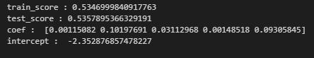
# 서초
area = '서초'
data = basic_df[basic_df['지역']==area]

x = data[['년도', '전용면적(㎡)', '층', '건축년도', '연도별 2030 거래비율']]
y = data['거래금액(만원)']
x_train, x_test, y_train, y_test = train_test_split(x, y, train_size=0.8, test_size=0.2)

model = LinearRegression()
model.fit(x_train, y_train)

coef.loc[area, :] = model.coef_

print('train_score :', model.score(x_train, y_train))
print('test_score :', model.score(x_test, y_test))

print('coef : ', model.coef_)
print('intercept : ', model.intercept_)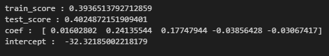
# 강남
area = '강남'
data = basic_df[basic_df['지역']==area]

x = data[['년도', '전용면적(㎡)', '층', '건축년도', '연도별 2030 거래비율']]
y = data['거래금액(만원)']
x_train, x_test, y_train, y_test = train_test_split(x, y, train_size=0.8, test_size=0.2)

model = LinearRegression()
model.fit(x_train, y_train)

coef.loc[area, :] = model.coef_

print('train_score :', model.score(x_train, y_train))
print('test_score :', model.score(x_test, y_test))

print('coef : ', model.coef_)
print('intercept : ', model.intercept_)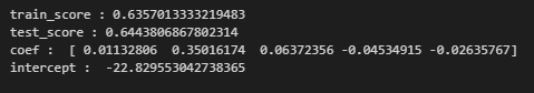
5-3. 노원구 실거래가에 진짜 2030 거래비율 영향이 클까?
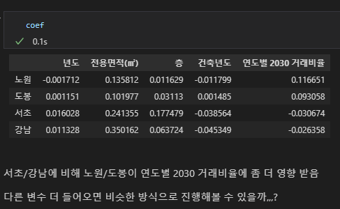
그렇긴 하대
'[패스트캠퍼스] 데이터분석부트캠프 > Python' 카테고리의 다른 글
| [7주차] Python: 데이터 분석 미니 프로젝트_사전 자료조사 (0) | 2023.04.16 |
|---|---|
| [6주차] Python: 크롤링 (0) | 2023.03.31 |
| [5주차] Python: List (0) | 2023.03.23 |
| [5주차] Python: 제어문(if, elif, else) (0) | 2023.03.23 |
| [5주차] Python: 파이썬 데이터 타입, 변수 (0) | 2023.03.23 |